Solving a real problem on quantum computers

This is the final of a series of four articles based on my Jupyter Notebooks exploring quantum computing as a tool for generating random number distributions.

Generating random numbers from a variety of specific probability distributions is interesting, and so is implementing digital computer operations on a quantum computer so that multiple operations are performed simultaneously. However neither of these is enough to justify the hype around quantum computers. Let’s now take a look at an example of something where quantum computers can significantly outperform digital computers. It’s known as Grover’s algorithm, and allows a quantum computer to take a function that might be performed on digital computers, and wraps it in some quantum goodness that quickly solves for it. “Solving for it” in this context means creating a probability distribution that is skewed in a controlled way so that the right answer comes up most often when measuring the qubits at the end.

Also, we will solve for a function of the type where it has one (or just a couple) of solutions, and where the approach to solve for it on a digital computer would be to “brute force” the answer by trying every possible solution to check if it works. On a quantum computer, there are some tricks to try the function fewer times, or even just once, and yet still figure out the solution. This demonstrates quantum advantage for using a quantum computer to solve problems of this type.

Functions of the type we’re interested in, that have one specific solution, exist all over the place. So, this is a potentially highly useful application for quantum computers. For example, a function that checks a possible set of numbers to a particular Sudoku puzzle to verify if it is a correct solution, a function that checks a password to see if it matches an encrypted password entry for a user, or a function that confirms the colour of a particular pixel in an image is correct for a given 3D scene with a particular set of objects and lighting. Many different problems can be rewritten in terms of a function that checks if a given answer is correct.

However, before seeing how to do this on a quantum computer, we need to introduce a couple of new operations.

Z operation

The Z operation works on all pairs of rows in the state vector associated with outcomes where there are different values of only a particular qubit, and flips the sign on the second row of each pair. We can call it the “flip” operation. Let’s have a quick look at an example.

In a two qubit scenario, if we start with an H(0) operator and an H(1) operator, as we did in the first notebook, we have the same value on each row of the state vector. If we then do a Z(0) followed by a Z(1), you can see the signs flip but the numbers otherwise stay the same.

QubitsInitial state vectorH(0)H(1)Z(0)Z(1)
|00>1.01/√21/21/21/2
|01>0.01/√21/2-1/2-1/2
|10>0.00.01/21/2-1/2
|11>0.00.01/2-1/21/2

We saw negative probabilities in the article where we introduced the RY operation, and here they are again. They are the key to how Grover’s algorithm works.

Note that we could have created a Z operation out of the operations that we already have, using a neat trick. The Z operation produces the same result as using the H, X, and H operations in sequence. If you remember, H takes a pair of rows with values a and b, and turns them into (a+b)/√2 and (ab)/√2. X then swaps these, so performing H again results in the pair of rows becoming 2a/(√2 x √2) and -2b/(√2 x √2) – which is just a and –b. However, Z is a common enough thing to want to do that it is useful to have it as a standalone operation rather than do H, X and H each time.

CCZ operation

Similarly to CCX, the CCZ operation is “doubly constrained”. In this case, it is a “doubly constrained flip” operation. Constrained to just those rows where the two specified qubits are |1>, it flips the sign of the second row of all pairs where the third qubit is the only one changing. Since the second row of these pairs is also the row where the third qubit is |1>, another way to think about this operation is flipping the sign of all rows where the three specified qubits are |1>.

Here’s an example of CCZ in practice:

QubitsInitial state vectorH(0)H(1)H(2)CCZ(0, 1, 2)
|000> (|0>)1.01/√21/21/√81/√8
|001> (|1>)0.01/√21/21/√81/√8
|010> (|2>)0.00.01/21/√81/√8
|011> (|3>)0.00.01/21/√81/√8
|100> (|4>)0.00.00.01/√81/√8
|101> (|5>)0.00.00.01/√81/√8
|110> (|6>)0.00.00.01/√81/√8
|111> (|7>)0.00.00.01/√8-1/√8

Implementing a verifier

The other thing that Grover’s algorithm needs is a function that verifies whether a value is a valid solution to some problem. All it needs to do is take a potential solution, and tell us “yes” or “no”.

We can do this by considering some of the qubits in the outcome to represent a proposed solution, and one other qubit to represent “yes” if it is |1> or “no” if it is |0>. In the example implemented here, qubits 0 and 1 will represent potential solutions, and qubit 2 will represent the result of validating it.

On a digital computer, we would think about this as bits. We would implement some logical operations that take two bits representing potential solutions and return another bit with the validation result. As we saw in the last notebook, we can implement the deterministic operations of a digital computer on a quantum computer by using X, CX, CCX, etc. operations.

Let’s say we want our verifier function to take state vectors where one of |000>, |001>, |010>, or |011> rows has the value 1.0 (100%), and only if it’s the “right” one, will the state vector be changed so that the corresponding row where qubit 2 is |1> becomes 1.0. For example, if |011> is the right solution, this would be implemented simply with the function CCX(0, 1, 2) which would swap the 1.0 value from |011> over to |111>.

Firstly, let’s use X operations to encode the value 3 into the state vector, by putting the value 1.0 in the |011> (|3>) row. (You can grab the complete Python script from here, or just type in the code below.)

import numpy as np
from qiskit import QuantumCircuit, QuantumRegister, ClassicalRegister, execute, BasicAer
from qiskit.visualization import plot_histogram
from qiskit.quantum_info import Statevector
import matplotlib.pyplot as plt
backend = BasicAer.get_backend('qasm_simulator')

q = QuantumRegister(3)    # We want 3 qubits
algo1 = QuantumCircuit(q) # Construct an algorithm on a quantum computer

# Start in the |3> row
algo1.x(0)
algo1.x(1)

v1 = Statevector(algo1)
print(np.real_if_close(v1.data))

$$\begin{bmatrix}
0.0 \\
0.0 \\
0.0 \\
1.0 \\
0.0 \\
0.0 \\
0.0 \\
0.0
\end{bmatrix}$$

Now if we perform CCX(0, 1, 2), the values in |011> (|3>) and |111> (|7>) will be swapped, moving the 1.0 value to the final row, where qubit 2 has a value of |1> . Since we know that CCX is constrained to work only on these rows, we know that only where the |011> potential solution is given the 1.0 value will the state vector be changed to have 1.0 on a row where qubit 2 is |1>. The other three potential solutions will result in no change.

# Apply CX operation, constrained to rows where qubit 0 and 1 are |1>, 
# swapping qubit 2's rows
algo1.ccx(0, 1, 2) 
v2 = Statevector(algo1)
print(np.real_if_close(v2.data))

$$\begin{bmatrix}
0.0 \\
0.0 \\
0.0 \\
0.0 \\
0.0 \\
0.0 \\
0.0 \\
1.0
\end{bmatrix}$$

To create different verifier functions, we can use X operations and specify either qubit 0 or qubit 1. For example, to create a function that will answer “yes” for the potential solution |01> and “no” the other three potential solutions, we simply do X(1) before doing CCX(0, 1, 2). We will also do X(1) again after the CCX to “undo” the first X, and ensure the state vector has 1.0 in the |101> (|5>) row:

QubitsInitial state vectorX(1)CCX(0, 1, 2)X(1)
|000> (|0>)0.00.00.00.0
|001> (|1>)1.00.00.00.0
|010> (|2>)0.00.00.00.0
|011> (|3>)0.01.00.00.0
|100> (|4>)0.00.00.00.0
|101> (|5>)0.00.00.01.0
|110> (|6>)0.00.00.00.0
|111> (|7>)0.00.01.00.0

Implementing this in Qiskit:

# Verifies that a proposed solution is correct only when it is |10>
def add_verify(algo):
    algo.x(1)
    algo.ccx(0, 1, 2)
    algo.x(1)

algo2 = QuantumCircuit(q) # Construct an algorithm on a quantum computer

# Ensure the state vector has 100% in the |001> row
algo2.x(0) 

add_verify(algo2) # Add the verify function to the algorithm
v3 = Statevector(algo2)
print(np.real_if_close(v3.data))

$$\begin{bmatrix}
0.0 \\
0.0 \\
0.0 \\
0.0 \\
0.0 \\
1.0 \\
0.0 \\
0.0
\end{bmatrix}$$

However, we need to modify the verifier function a little before we use it in Grover’s algorithm. We are going to apply the H operation on the result qubit (qubit 2) before running the function, and then again afterwards.

This is a little trick that turns an X operation into a Z operation. So, the CCX operation effectively becomes like a CCZ operation. And yes, the verifier function could have just been written with a CCZ instead of a CCX and we could skip the H operations, but digital computer operations don’t use Z type operations, and this way the algorithm is more general.

# Flips the sign of the row corresponding to the outcome that 
# the verify function would indicate is correct
def add_verify_with_h(algo):
    algo.h(2)
    add_verify(algo)
    algo.h(2)

This version of the function will now flip the sign of the state vector row with the answer, so if the state vector was fully populated with positive values, the solution will be revealed as the one that’s negative. Unfortunately, we can’t stop here with the job done, because in practice we can’t read the state vector out of the quantum computer. All we can do is take measurements of the qubits, and while we can have a negative value in a row of a state vector, we won’t see a negative probability appear in measurements.

Grover’s algorithm is about amplifying the negative row so it will have a higher probability in the measurements.

Grover’s algorithm

Normally the verification function will be quite complicated, and difficult to figure out from just looking at it. Our verification function is simple, but that’s fine for learning how Grover’s algorithm works.

The basic strategy for using Grover’s algorithm is to:

  1. Prepare the state vector so it has the same value on every row, i.e. no row has a zero value.
  2. Apply the verification function, which will flip the sign of the row corresponding to the right answer.
  3. Amplify the negative rows compared to the non-negative rows.

Then we measure the qubits, and the most likely result should be the right answer. For larger numbers of qubits, the steps 2 and 3 will typically be repeated to make the right answer clearer, but we shouldn’t need to do that for our example.

We’ve already defined the verification function, but here’s the state preparation function:

# Creates a uniform probability distribution across the state vector
def add_prepare(algo):
    algo.h(0)
    algo.h(1)
    algo.h(2)

It is just the approach to creating a uniform probability distribution that we saw in the first notebook.

We can see how the verification function just flips the sign of the answer row |101> when given a state vector with 1/√8 values in all of its rows:

algo3 = QuantumCircuit(q) # Construct an algorithm on a quantum computer
add_prepare(algo3)        # Add the operations to prepare the state vector
add_verify_with_h(algo3)  # Add the sign-flipping version of verify 
v4 = Statevector(algo3)
print(np.real_if_close(v4.data))

$$\begin{bmatrix}
\frac{1}{\sqrt{8}} \\
\frac{1}{\sqrt{8}}\\
-\frac{1}{\sqrt{8}} \\
\frac{1}{\sqrt{8}} \\
\frac{1}{\sqrt{8}}
\end{bmatrix}$$

Step 3 – the amplification function – requires a bit of explanation.

The idea now is to make everything a bit more negative, and because one row is already negative, that row becomes much more negative than the other rows. As the probability that the outcome of a measurement being a given row is equal to the square of the value of that row, it doesn’t matter than the values are negative. The row that is more negative than the other rows will end up becoming a more likely outcome.

The workhorse of the procedure is the H operation. As we discussed in the first notebook, it is like a “half” operation, where it works on all pairs of rows that differ only by a specific qubit, and turns the first of these into the sum of the pairs divided by the root of a half, and the second into the difference of the pairs divided by the root of a half.

There are two observations worth noting here. Firstly, it puts the sums of the pairs into the first row, i.e. the row where the specific qubit has a |0> outcome. Secondly, it is its own inverse, i.e. that it you perform two identical H operations in sequence, the second operation undoes the first one.

Using these two observations, the amplification function applies the H operation for each of the qubits in turn, resulting in all rows being summed into the first row of the state vector, i.e. corresponding to the |000> outcome, although this sum will be divided by the root of 8, which is the result of dividing by √2 in the calculations three times. However, this row will be a large, positive value compared to the others.

Then the amplification function flips the sign on the |000> row, making it a large, negative value. Lastly, the H operation is applied for each qubit in turn, reversing the earlier H operations, but spreading the amount “taken” from the |000> row evenly across all of the rows.

Let’s see it in action. Firstly, let’s apply H for each qubit. We can do this by reusing the prepare function:

add_prepare(algo3)
v5 = Statevector(algo3)
print(np.real_if_close(v5.data))

$$\begin{bmatrix}
3/4 \\
1/4 \\
-1/4 \\
1/4 \\
1/4 \\
-1/4 \\
1/4 \\
-1/4
\end{bmatrix}$$

After the verify function was performed, all rows were 1/√8, except for the solution row which was negative. The sum of all rows is 6/√8 and this value divided by √8 is 3/4, which is what we’ve ended up with in row |000> after the first part of the amplification procedure.

Next we flip the sign on that row so it becomes negative. We have an operation – CCZ – that flips the sign on the |111> row, but not one for the |000> row. Still, we can do this by first using the X operation for each qubit, to reverse the order of the state vector. On a digital computer, to reverse a vector like this, you’d need to perform an operation for each row in the first half of the vector, swapping it with its counterpart row in the second half of the vector. Quantum computers are much more efficient at this.

X(0) swaps groups of rows separated by one row, X(1) swaps groups of rows separated by two rows, and X(2) swaps groups of rows separated by four rows. Once we’ve performed each of these, the state vector has been reversed:

# Reverses the rows of the state vector
def add_reverse(algo):
    algo.x(0)
    algo.x(1)
    algo.x(2)

Using this reverse routine, we can following it by using CCZ to flip the sign on row |111>, then reverse the state vector again to put the state vector back in the original order.

add_reverse(algo3) # Add the operations to reverse the state vector
algo3.ccz(0, 1, 2) # Apply the CCZ operation to flip the sign on row |111>
add_reverse(algo3) # Add the operations to reverse the state vector again
v6 = Statevector(algo3)
print(np.real_if_close(v6.data))

$$\begin{bmatrix}
-3/4 \\
1/4 \\
-1/4 \\
1/4 \\
1/4 \\
-1/4 \\
1/4 \\
-1/4
\end{bmatrix}$$

Note that in flipping the sign on the 3/4 value in row |000>, we have effectively deducted an amount equal to 6/4 (or 3/2) from this row. This reduction will now be spread back across all the rows by using the H operation for each qubit again.

add_prepare(algo3)
v7 = Statevector(algo3)
print(np.real_if_close(v7.data))

$$\begin{bmatrix}
-\frac{1}{\sqrt{32}} \\
-\frac{5}{\sqrt{32}} \\
-\frac{1}{\sqrt{32}} \\
-\frac{1}{\sqrt{32}}
\end{bmatrix}$$

The reduction by 3/2 has been divided by √8 again, so the difference between these values and the ones after the verify function is just 3/√32. All of the rows that were 1/√8 are now -1/√32, and the single row that was -1/√8 is now -5/√32. If you’re following along with Python yourself, the output probably doesn’t show it, and just shows -0.17678 (or similar) for all rows except one that shows -0.88388 (or similar).

Now that we’ve worked through the operation of the amplify function, we can define it as a Python function:

# Amplifies the row with a negative value to become more negative
def add_amplify(algo):
    add_prepare(algo)
    add_reverse(algo)
    algo.ccz(0, 1, 2)
    add_reverse(algo)
    add_prepare(algo)

Let’s now see the whole thing in action, and what gets measured at the end. (You can grab a simplified version of the Python script from here that does only this bit, or just type in the code below.)

c = ClassicalRegister(2)     # The solution at the end has only 2 bits
algo4 = QuantumCircuit(q, c) # Construct an algorithm on a quantum computer

add_prepare(algo4)           # Step 1 of Grover's: prepare the state vector
add_verify_with_h(algo4)     # Step 2 of Grover's: flip the solution row 
add_amplify(algo4)           # Step 3 of Grover's: amplify negative rows

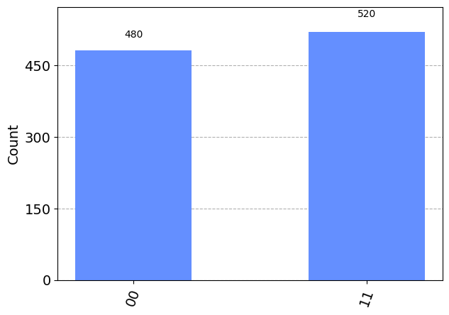
algo4.measure(q[0:2], c)     # Measure the two qubits 0 and 1, get some bits
result = execute(algo4, backend, shots=1000).result() # Run this all 1,000 x
plot_histogram(result.get_counts(algo4))              # Show a histogram 
plt.show()

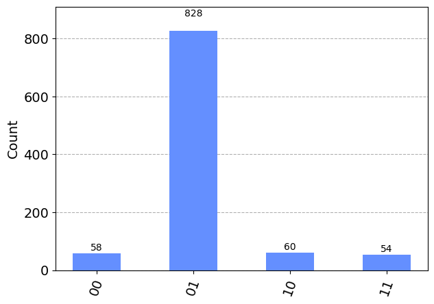
You can go back and set up the verify function differently, and you’ll see that the algorithm will still reveal the correct solution in the measurements.

In this way, the quantum computer hasn’t needed to brute force the answer by trying the verification function over and over again until it finds the answer. The fact that the verification function can be used to make a row in the state vector negative was enough to allow this negative value to be amplified, and set up a probability distribution that makes the answer pop out more often in the measurements.

As I mentioned at the start, it may be that the

add_verify_with_h(algo4)
add_amplify(algo4)

steps need to be repeated as the number of qubits increases. However, it won’t need to be done as frequently as once per qubit, so it will continue to be more efficient than the brute force approach that a digital computer has to use.

In conclusion

We added another two operations to our set, and have seen how to use them on a quantum computer to quickly figure out the solution to the digital computing function that verifies solutions to a problem. Here is the complete set of operations over these four articles:

OperationShort-hand descriptionSpecified byDetailed description
H“half”1 qubitFor all pairs of rows that differ only by the value of a specific qubit in the outcome, replace the first row value with a new value that is the sum of the original values divided by √2, and the second row value with the difference between the original values divided by √2.
CX“constrained swap”2 qubitsFor all pairs of rows where the first qubit specified is in the |1> state in the outcome, and where otherwise the rows differ only by the value of the second qubit specified, swap the rows in the pair.
RY“relative swap”1 angle and 1 qubitFor all pairs of rows that differ only by the value of a specific qubit in the outcome, swap a fraction “f” of the value from the first row to the second, and bring the opposite fraction (i.e. 1-f) from the second row but with the sign flipped, where “f” is specified as the angle 2 x arcsin(√f). If “f” is 1.0, the angle will be 𝜋.
X“swap”1 qubitFor all pairs of rows that differ only by the value of a specific qubit in the outcome, swap the values in the pair.
CCX“doubly constrained swap”3 qubitsFor all pairs of rows where both the first and second qubit specified are in the |1⟩ state in the outcome, and where otherwise the rows differ only by the value of the third qubit specified, swap the rows in the pair
Z“flip”1 qubitFor all pairs of rows that differ only by the value of a specific qubit in the outcome, flip the sign on the second row of each pair.
CCZ“doubly constrained flip”3 qubitsFor all pairs of rows where both the first and second qubit specified are in the |1> state in the outcome, and where otherwise the rows differ only by the value of the third qubit specified, flip the sign on the second row of each pair.

That’s all for now. Hope you’ve enjoyed working along with me in seeing how quantum computers can perform computation by changing the probabilities of the different possible outcomes of their qubits, and how often this approach allows quantum computers to solve a problem more efficiently than a digital computer.

Digital operations on quantum computers

This is the third in a series of four articles based on my Jupyter Notebooks exploring quantum computing as a tool for generating random number distributions.

Generating random numbers from a variety of specific probability distributions shows us how the quantum state vector reflects the desired probability distribution, and the previous article showed how a variety of such distributions could be achieved. However, quantum computers can simulate a digital computer also. Even though bits are certain and qubits are uncertain, computing on a digital computer can be thought of like working with a special kind of probability distribution: one where there is a row on the state vector with a 100% probability, and all the rest are zero. This reflects how digital computers are deterministic.

Let’s look at how we might perform digital computing operations on a quantum computer, sticking with high-school level maths. First, we need to introduce some new operations.

X operation

We have already seen the CX, or “constrained swap”, operation. There is a simpler one called the X operation which does a swap within all pairs of rows in the state vector where the only difference is in a specific qubit. So, where the CX operation required specifying two qubits to determine the rows it affects, the X operation requires specifying just one qubit. Where you might think of CX as a “constrained swap”, you can think of X as just a “swap”.

To clarify the X operation, here is an example of how it might be used:

QubitsInitial state vectorX(0)X(1)
|00>1.00.00.0
|01>0.01.00.0
|10>0.00.00.0
|11>0.00.01.0

The first X swaps the first two rows, as these differ only in qubit 0 (the rightmost qubit), and while it also swaps the second two rows, these were the same, so we don’t see a difference there. The second X swaps rows |01> and |11>, as these differ only in qubit 1 (the leftmost qubit), and while it also swaps the remaining two rows, again these were the same value, so we don’t see any difference after the operation.

CCX operation

Now that we know about X and CX, you might be wondering if there are more constraints that can be added to X. Yes, a common operation is a “doubly constrained” version of X, sometimes known as a Toffoli operation.

The CCX operation is constrained to operate only on pairs of rows where two specified qubits are |1>, and it swaps pairs of rows where only a third qubit changes, i.e. a “doubly constrained swap” operation. Here’s what some CCX operations look like on a state vector consisting of three qubits:

QubitsInitial state vectorX(1)CCX(0, 1, 2)X(0)CCX(0, 1, 2)
|000> (|0>)1.00.00.00.00.0
|001> (|1>)0.00.00.00.00.0
|010> (|2>)0.01.01.00.00.0
|011> (|3>)0.00.00.01.00.0
|100> (|4>)0.00.00.00.00.0
|101> (|5>)0.00.00.00.00.0
|110> (|6>)0.00.00.00.00.0
|111> (|7>)0.00.00.00.01.0

Since our examples use Qiskit, qubits are numbered from the right. Qubit 0 is the rightmost one, then qubit 1 is in the middle, and qubit 2 is the leftmost one. In the above table, as it is starting to get long, next to the qubits identifier for the row, I’ve also written the row number in brackets. The qubits identifier is a binary number, and corresponds to a decimal number, which is the row number, e.g. “011” is the binary number for 3, so I’ve written this as |011> (|3>).

In this example, the CCX(0, 1, 2) operation swaps rows where qubits 0 (rightmost) and 1 (middle) are |1>, i.e. those rows ending in |11>: rows |3> and |7>. The first time this operation is performed, both of those rows are 0.0, so it looks like nothing happens, but the second time, we see the effect of the swap performed.

Incrementing a 3-bit number

A very common operation on a digital computer is incrementing a number, or in other words, adding one to it. Incrementing 3 results in 4, incrementing 6 results in 7, and so on.

Each row of the state vector represents a different number, i.e. the decimal number corresponding to the binary number for that arrangement of qubits. For a state vector that represents 3 qubits, row |100> is row |4>, while row |110> is row |6>. Incrementing a number can be thought of as taking a state vector with a specific number encoded in it – the row with 100% probability – and turning it into a state vector with a new number encoded in it, specifically the original number plus one. For example, if we start with a state vector with row |4> with 100% probability, incrementing this would result in a new state vector with row |5> having 100% probability.

To implement this sort of algorithm, where a row has 100% probability, and we make another row 100% probability, we simply need to use variants of the X operation. The X, CX and CCX operations only swap rows around, so will always leave the state vector having a single row with 100% probability. In this case, they can simulate the deterministic operations of a digital computer.

To increment a number encoded on the state vector using variants of the X operation, it is quite straightforward, but we need to think about it in binary notation. If we add one to a number ending in |0>, it becomes |1>. While if we add one to a number ending in |1>, it will become |0> and carry a one to the next place. To achieve this, we can use X to swap from a row |0> to a |1> row, or visa versa, and a CX to manage the carrying of the one. Similarly, we can use a CCX to manage the carrying of the one to the final place.

Implementing in Qiskit

Let’s create this increment operation as a Python function. (You can grab the complete Python script from here, or just type in the code below.)

import numpy as np
from qiskit import QuantumCircuit, QuantumRegister, ClassicalRegister
from qiskit.quantum_info import Statevector

# Add the operations to an algorithm that increments the number 
# encoded on a 3 qubit state vector
def add_increment(algo):
    algo.ccx(0, 1, 2) # Carry the one to qubit 2, when qubits 0 and 1 are |11>
    algo.cx(0, 1)     # Carry the one to qubit 1, when qubit 0 is |1>
    algo.x(0)         # Add one to qubit 0

Now we can test it out.

q = QuantumRegister(3)    # We want 3 qubits
algo1 = QuantumCircuit(q) # Construct an algorithm on a quantum computer

# Start in the |2> row
algo1.x(1)
v1 = Statevector(algo1)
print(np.real_if_close(v1.data))

$$\begin{bmatrix}
0.0 \\
0.0 \\
1.0 \\
0.0 \\
0.0 \\
0.0 \\
0.0 \\
0.0
\end{bmatrix}$$

# Increment the number encoded in the state vector
add_increment(algo1)
v2 = Statevector(algo1)
print(np.real_if_close(v2.data))

$$\begin{bmatrix}
0.0 \\
0.0 \\
0.0 \\
1.0 \\
0.0 \\
0.0 \\
0.0 \\
0.0
\end{bmatrix}$$

# Increment the number once more
add_increment(algo1)
v3 = Statevector(algo1)
print(np.real_if_close(v3.data))

$$\begin{bmatrix}
0.0 \\
0.0 \\
0.0 \\
0.0 \\
1.0 \\
0.0 \\
0.0 \\
0.0
\end{bmatrix}$$

We are successfully incrementing the number encoded in the state vector each time.

Doing multiple increments simultaneously

What if multiple numbers were encoded in the state vector? Actually, the same algorithm will continue to work.

Let’s start by encoding two numbers, so rather than one row having a 100% probability, the state vector will have two rows each with 1/√2 . Remember that we square this to get the probability, which will be 1/2 or 50%.

In Qiskit, we will encode both |0> and |3>, and apply the increment operation.

algo2 = QuantumCircuit(q) # Construct an algorithm on a quantum computer

# Start with |0> and |3> rows having equal probability
algo2.h(2)
v4 = Statevector(algo2)
print(np.real_if_close(v4.data))

$$\begin{bmatrix}
\frac{1}{\sqrt{2}} \\
0.0 \\
0.0 \\
0.0 \\
\frac{1}{\sqrt{2}} \\
0.0 \\
0.0 \\
0.0
\end{bmatrix}$$

# Increment the numbers encoded in the state vector
add_increment(algo2)

v5 = Statevector(algo2)
print(np.real_if_close(v5.data))

$$\begin{bmatrix}
0.0 \\
\frac{1}{\sqrt{2}} \\
0.0 \\
0.0 \\
0.0 \\
\frac{1}{\sqrt{2}} \\
0.0 \\
0.0
\end{bmatrix}$$

Now it has rows |1> and |4> with equal probability. Two increments have been performed simultaneously, without changing the increment operation at all. (In fact, the increment operation can also be thought of as a rotation operation, where the values are rotated through all of the rows of state vector, a row at a time.)

It is this sort of capability that highlights the power of quantum computers to rapidly speed up some types of computation.

In conclusion

We have added another two more operations to our set, and seen how to use them on a quantum computer to perform a traditional digital computer functions (incrementing a number). We’ve also seen how quantum computers can enhance digital functions, like performing multiple increments at once. Here is the set of operations we’ve talked about so far:

OperationShort-hand descriptionSpecified byDetailed description
H“half”1 qubitFor all pairs of rows that differ only by the value of a specific qubit in the outcome, replace the first row value with a new value that is the sum of the original values divided by √2, and the second row value with the difference between the original values divided by √2.
CX“constrained swap”2 qubitsFor all pairs of rows where the first qubit specified is in the |1> state in the outcome, and where otherwise the rows differ only by the value of the second qubit specified, swap the rows in the pair.
RY“relative swap”1 angle and 1 qubitFor all pairs of rows that differ only by the value of a specific qubit in the outcome, swap a fraction “f” of the value from the first row to the second, and bring the opposite fraction (i.e. 1-f) from the second row but with the sign flipped, where “f” is specified as the angle 2 x arcsin(√f). If “f” is 1.0, the angle will be 𝜋.
X“swap”1 qubitFor all pairs of rows that differ only by the value of a specific qubit in the outcome, swap the values in the pair.
CCX“doubly constrained swap”3 qubitsFor all pairs of rows where both the first and second qubit specified are in the |1⟩ state in the outcome, and where otherwise the rows differ only by the value of the third qubit specific, swap the rows in the pair

The next article will look at a well-known algorithm that performs a task that is complex on a digital computer but is very efficient on a quantum computer.

Further adventures in quantum randomness

This is the second in a series of four articles based on my Jupyter Notebooks exploring quantum computing as a tool for generating random number distributions.

The first article showed how a quantum computer could be programmed to generate a uniform random distribution of two bits using operations on qubits. It was a pretty trivial algorithm, and compared with the complexity of generating pseudo-random numbers on a digital computer, showed the advantage of using quantum computers for this application. However, given that I discussed how quantum computers can manipulate probabilities, it’s natural to consider how other, non-uniform, random number distributions might be calculated using a quantum computer. As with the first article, I’m sticking with high-school level maths.

Bell state

A special type of quantum state is known as the Bell state. There are actually four Bell states, but for simplicity, we’ll just pick one. To put a two qubit quantum computer into a Bell state, we will manipulate it to have the state vector

$$\begin{bmatrix}
\frac{1}{\sqrt{2}} \\
0.0 \\
0.0 \\
\frac{1}{\sqrt{2}}
\end{bmatrix}$$

which means that a measurement will get either the |00> or |11> outcomes with equal probability, but the |01> and |10> outcomes won’t appear at all. Another way to think of this is flipping two coins, and having them always end up heads-heads or tails-tails, but never getting a heads-tails result.

To get this state vector, it’s not enough to use the H operation, but we need something called the CX operation.

CX operation

The CX operation can be thought of as a “constrained swap” operation which affects pairs of rows in the state vector specified by the states of two qubits (rather than specified by just one qubit, like we saw with the H operation). It will cause the values of those pairs of rows to swap, constrained to those pairs of possible outcomes where the first qubit specified is in the |1> state and that otherwise differ only by the value of the second qubit.

For example, if we start with the usual initial state vector for two qubits:

QubitsInitial state vector
|00>1.0
|01>0.0
|10>0.0
|11>0.0

where the |00> outcome has a 100% probability, and now apply the CX operation against the right-most qubit then the left-most qubit, or CX(0,1) to use the Qiskit numbering for qubits, the state vector wouldn’t change at all, since the pair of rows where the right-most qubit is |1> are both the same, i.e. 0.0, so swapping doesn’t change anything.

However, if we firstly use the H operator on rows associated with the right-most qubit, or an H(0) operation, and then perform the same CX(0,1) operation, we get a more interesting result:

QubitsInitial state vectorWorking out H(0)Result of H(0)Working out CX(0,1)Result of CX(0,1)
|00>1.0=(1.0+0.0)/√21/√2unchanged1/√2
|01>0.0=(1.0-0.0)/√21/√2=0.00.0
|10>0.0=(0.0+0.0)/√20.0unchanged0.0
|11>0.0=(0.0-0.0)/√20.0=1/√21/√2

Swapping the rows made a change this time, and we have ended up with the Bell state that we were talking about above.

Implementing this on Qiskit

Now, let’s create a histogram of the results we get from performing this on a (simulated) quantum computer, and check that it does what we expect. We’ll use the same approach with Qiskit as we did last time. (You can grab the complete Python script from here, or just type in the code below.)

import numpy as np
from qiskit import QuantumCircuit, QuantumRegister, ClassicalRegister, execute, BasicAer
from qiskit.visualization import plot_histogram
import matplotlib.pyplot as plt
backend = BasicAer.get_backend('qasm_simulator')

q = QuantumRegister(2)   # We want to use 2 qubits
algo = QuantumCircuit(q) # Readies us to construct an algorithm to run on the quantum computer

algo.h(0)          # Apply H operation on pairs of rows related to qubit 0
algo.cx(0,1)       # Apply CX operation, constrained where qubit 0 is |1>
algo.measure_all() # Measure the qubits and get some bits

result = execute(algo, backend, shots=1000).result()
plot_histogram(result.get_counts(algo))
plt.show()

Yes, this is the random distribution we were hoping to get. It is just “00” and “11” with no “01” or “10” results.

RY operation

We’ve achieved a non-uniform distribution, but it’s not a very interesting one. It’s a 50-50 outcome, and we could have achieved that with 1 qubit. We didn’t really need 2 qubits. To create more interesting distributions, we will need another operation. Let’s take a look at the RY operation.

RY adjusts the pairs of state vector rows applying to a specified qubit, and adjusts them by a specified “angle”. If the angle is pi (𝜋), which is an amount in radians equivalent to 180 degrees, the adjustment results in a swap of values and flipping the sign of the first value (we’ll come back to this). But the swap is modified relative to the angle, so we can think of it like a “relative swap” operation.

Let’s have a look at at how it would work on the standard initial state vector, with the specific qubit being the right-most one (or, qubit 0), and for some different angles:

QubitsInitial state vectorR(0.0, 0)R(𝜋, 0)R(𝜋, 0) againR(𝜋/2, 0)
|00>1.01.00.0-1.0-1/√2
|01>0.00.01.00.0-1/√2
|10>0.00.00.00.00.0
|11>0.00.00.00.00.0

The first time the RY operation is used, it is given a specified angle of 0.0, and it does absolutely nothing to the state vector. This is correct – with an angle of 0.0, RY will not change anything.

Next, we can see that when the RY(𝜋, 0) operation happens, it swaps the values where the right-most qubit (qubit 0) differ, i.e. the first and second row, and the third and fourth row. In addition, it flips the sign on the first of each pair of rows. The first time RY happens, it simply moves the 100% outcome from |00> to |01>. The second time RY happens, it moves this outcome back to |00> and flips the sign to negative.

What does -100% mean? How can this be a probability? Well, each row of the state vector is a probability amplitude rather than a probability. If a probability amplitude is a real number, i.e. no imaginary component, you can turn it into its corresponding probability by just squaring it. -1.0 x -1.0 is 1.0, so -100% as a probability amplitude is equivalent to a 100% probability. Note that this isn’t just some oddity, but actually part of what makes quantum computers powerful.

The final application of the RY operation in the table is with a specified angle that is 𝜋/2 which corresponds to 90 degrees. It’s mid-way between 0.0 and 𝜋, and produces a result that is also mid-way between the previous results. Where the 0.0 angle didn’t move any of the probability amplitude values between the pairs, and the 𝜋 angle moved all of the probability amplitude values to the alternate row in each pair, the 𝜋/2 angle is halfway between those angles and it moved half the probability amplitude, in the same way the H operator did in the previous notebook.

In fact, we can pick an angle to give to the RY operation that will move a desired fraction of the probability amplitude value between the rows. To swap a fraction “f” of the value from the first row to the second, and bring the opposite fraction (i.e. 1-f) from the second row but with the sign flipped, you use the angle calculated by 2 x arcsin(√f). For our final application of RY above, it had the fraction f=1/2, and it turns out that 2 x arcsin(√(1/2)) = 𝜋/2 which is the angle used in the operation.

We can now use this knowledge to create a range of specific probability distributions for our random bits. The set of operations we have talked about so far – H, CX and RY – should allow us to create any probability distribution. For example, if we want to create a probability distribution where it is equally likely that any of the first three outcomes (|00>, |01>, and |10>) happen and yet the last outcome (|11>) shouldn’t happen, the state vector we’d want to create is:

$$\begin{bmatrix}
\sqrt{\frac{1}{3}} \\
0.0
\end{bmatrix}$$

A way to get this is to recognise that if we look at the state vector as two pairs of rows, the first pair of outcomes are twice as likely in total as the second pair of outcomes. We can use the RY operation to swap (the square root) of a third of the overall probability to the second pair. We can then use a sequence of H, RY, CX and RY operations to spread the probabilities within each pair. This looks like:

QubitsInitial state vectorRY(2 x arcsin(√(1/3)), 1)H(0)RY(𝜋/4, 0)CX(1, 0)RY(-𝜋/4, 0)
|00>1.0√(2/3)√(1/3)0.31250.3125√(1/3)
|01>0.00.0√(1/3)0.75430.7543√(1/3)
|10>0.0√(1/3)√(1/6)0.22090.5334√(1/3)
|11>0.00.0√(1/6)0.53340.22090.0

You can see here that after the H(0) operation, the first two rows have the values we want, but the final two rows had the desired values before the H(0). The operations following the H(0) have the effect of undoing the H(0) operation on the final two rows but leaving the first two rows alone. Note that the final two RY operations are opposite signs to each other, so they should cancel each other out, but a CX(1,0) operation has been done in the middle. This CX operation, in swapping the final two rows, has the effect of making it as if the first of the final two RY operations was also a negative angle for those rows, so instead of cancelling out (like happened on the first two rows), the two RY operations on those rows add together as if it was an RY operation of -𝜋/2. As we saw above, an RY operation with the angle 𝜋/2 is similar to an H operation, and with the negative angle, the RY operation acts to reverse the H.

Don’t worry if you didn’t fully follow that. This sort of procedure is called “amplitude embedding” or “state preparation”, and there are various algorithms to do this, many of which get quite esoteric. The above procedure was inspired by a paper by Mottonen, Vartiainen, Bergholm, and Salomaa. The main thing to note is that quantum computers allow arbitrary non-uniform distributions to be constructed.

Implementing this on Qiskit

Let’s test the above procedure and see if it does what we expect. (You can grab the complete Python script from here, or just type in the code below.)

import numpy as np
from qiskit import QuantumCircuit, QuantumRegister, ClassicalRegister, execute, BasicAer
from qiskit.visualization import plot_histogram
import matplotlib.pyplot as plt
backend = BasicAer.get_backend('qasm_simulator')

q = QuantumRegister(2)   # We want to use 2 qubits

angle1 = 2 * np.arcsin(np.sqrt(1.0/3.0))
angle2 = np.pi / 4

algo = QuantumCircuit(q) # Readies us to construct an algorithm to run on the quantum computer

algo.ry(angle1, 1)       # Apply RY operation to swap 1/3 of qubit 1's value 
algo.h(0)                # Apply H operation on pairs of rows related to qubit 0
algo.ry(angle2, 0)       # Apply RY operation to perform a half of H on qubit 0
algo.cx(1,0)             # Apply CX operation, constrained to where qubit 1=|1>
algo.ry(-angle2, 0)      # Apply RY operation to undoing half of H on qubit 0

algo.measure_all()       # Measure the qubits and get some bits

result = execute(algo, backend, shots=1000).result()
plot_histogram(result.get_counts(algo))              
plt.show()

This is exactly what we were hoping to see. It is “00”, “01” and “10” split three ways, and with no “11” results.

In conclusion

We have added two more operations to our set, and seen how to use them on a quantum computer to create a variety of random distributions, such as the Bell state:

OperationShort-hand descriptionSpecified byDetailed description
H“half”1 qubitFor all pairs of rows that differ only by the value of a specific qubit in the outcome, replace the first row value with a new value that is the sum of the original values divided by √2, and the second row value with the difference between the original values divided by √2.
CX“constrained swap”2 qubitsFor all pairs of rows where the first qubit specified is in the |1> state in the outcome, and where otherwise the rows differ only by the value of the second qubit specified, swap the rows in the pair.
RY“relative swap”1 angle and 1 qubitFor all pairs of rows that differ only by the value of a specific qubit in the outcome, swap a fraction “f” of the value from the first row to the second, and bring the opposite fraction (i.e. 1-f) from the second row but with the sign flipped, where “f” is specified as the angle 2 x arcsin(√f). If “f” is 1.0, the angle will be 𝜋.

The next article will look at how to implement digital computing functions through operations on the state vector.

A Quantum Computer is a random number generator

This is the first in a series of four articles based on my Jupyter Notebooks exploring quantum computing as a tool for generating random number distributions.

Many of the introductory quantum computing articles and courses out there are not quite right. They either quickly head deep into details that require a University-level physics or mathematics background, or sit at a high level based on analogies that are out of step with how quantum computers actually work. I want to try something different, and introduce some useful quantum computing algorithms using high-school level maths. I will avoid much (but maybe not all) of the jargon, and show how the algorithms can be implemented on the commonly available Qiskit platform.

In my earlier article on quantum computing, I introduced an analogy to describe quantum computers, which are based on qubits rather than bits. The analogy was of a coin-flipping robot arm that is flipping a coin that lands on a table. A qubit is like the coin when it is in the air, and a bit is like the coin when it has ended up on the table. When it’s in the air, the coin is in a kind of probabilistic state where it may end up heads or tails, but once it’s on the table, it’s in a certain state where it is definitely one of either heads or tails. Quantum computers work in the realm of probabilities, and can manipulate the coin while it’s still spinning in the air. The spinning coin in the air is the qubit. But at some point it will land on the table and be measured as either heads or tails. At that point it becomes a bit.

To write about quantum states, a notation is used where the name of the state is put between a vertical bar and an angle bracket. Just like a single bit can be in the “0” state or the “1” state, for a single qubit, we might say it can be in the |0> state or the |1> state. Our hypothetical robot-arm is well-calibrated, so it consistently flips a coin that lands with the same side facing up, and the resulting coin is like having a qubit in one of these states. The coin is in a probabilistic state, but the probability of it having a particular result is 100%. Similarly, if a qubit is in the |0> state, when it is measured, you will get a “0” result 100% of the time.

However, a quantum computer can manipulate the probabilities of the qubit, so even if the qubit started in the |0> state, after manipulation it enters a new state where if the qubit is measured, it will get “0” outcome 50% of the time (and “1” outcome the other 50% of the time, of course). This is done using a Hadamard operation, usually just written as H. We will use this operation to create truly random numbers.

Creating truly random numbers

Mostly when you have a computer give you a random number, such as using the RAND function in Microsoft Excel or when you’re playing a computer game and the enemy does something unexpected, the computer is actually producing a pseudo-random number. If you could create a perfect snapshot of everything in your computer, then get it to do something “random”, and return to that snapshot again, it will do exactly the same random thing each time. So, it’s not actually random, but it looks random unless you peer too closely.

For most applications, that’s fine. But if you are doing cryptography, having truly random numbers is important. You want to generate a secret key that no-one else can guess. Ideally, even if someone could take a snapshot of your computer, they still couldn’t predict what secret key is generated. There are special hardware random number generators that can create truly random numbers (Cloudflare uses lava lamps!), and quantum computers create truly random numbers too.

Let’s say we are going to generate a 2 bit random number. We’ll use 2 qubits, and the starting state of the qubits will be |00>, which means the outcome of measuring them both as “0” is 100%. We’ll use a quantum computer to manipulate the qubits so that all four possible outcomes |00>, |01>, |10>, or |11> are equally likely. Then when the qubits are measured, we will have some truly random bits.

We can write the four possibilities as a vector, with each row consisting of the probability of that outcome. Quantum computers perform their calculations using complex numbers rather than real numbers, and this is because complex numbers are needed to accurately describe how things work at the quantum level. We can simplify things, and just use real numbers, but we will need to calculate probabilities by squaring the values in each row of the vector.

We call this vector the quantum state vector (or just state vector), and it starts with being

$$\begin{bmatrix}
1.0 \\
0.0 \\
0.0 \\
0.0
\end{bmatrix}$$

Each row of the state vector corresponds to a different outcome, with the outcomes for two qubits being |00>, |01>, |10>, and |11> as we go down the vector. So this state vector represents a 100% probability of getting the |00> outcome.

We want each outcome to have a 25% probability, so we want to change the state vector to be:

$$\begin{bmatrix}
\frac{1}{2} \\
\frac{1}{2} \\
\frac{1}{2} \\
\frac{1}{2}
\end{bmatrix}$$

Of course, when you square 1/2, you get 1/4, or 25%.

The H operation is a standard operation on quantum computers, and works on all pairs of rows of the quantum state vector where that outcome differs only by the value of a specific qubit, e.g. where one outcome has the |0> for that qubit and the other row has |1>. For each pair, it turns the first value into a new value that is the sum of the original values divided by \(\sqrt{2}\), and the second value into the difference between the original values divided by \(\sqrt{2}\). While it is a division by \(\sqrt{2}\) rather than a division by 2, you can think of H like a “half” operation, where it calculates half the sum and half the difference and is scaled by a normalisation constant so that when the values are squared, the probabilities add up to 1.0. Written out mathematically, if the first row value is \(a\) and the second row value is \(b\), the first row value becomes \(\frac{a+b}{\sqrt{2}}\) and the second row value becomes \(\frac{a-b}{\sqrt{2}}\).

To get the desired final state vector from the initial state vector, we can apply H first to the pair of rows associated with a difference in the right-most qubit, then apply H to the pair of rows associated with a difference in the left-most qubit. Here’s how it would go:

QubitsInitial state vectorWorking out first HResult of first HWorking out second HResult of second H
|00>1.0=\(\frac{1.0+0.0}{\sqrt{2}}\)\(\frac{1}{\sqrt{2}}\)=\(\frac{\frac{1}{\sqrt{2}}+0.0}{\sqrt{2}}\)\(\frac{1}{2}\)
|01>0.0=\(\frac{1.0-0.0}{\sqrt{2}}\)\(\frac{1}{\sqrt{2}}\)=\(\frac{\frac{1}{\sqrt{2}}-0.0}{\sqrt{2}}\)\(\frac{1}{2}\)
|10>0.0=\(\frac{0.0+0.0}{\sqrt{2}}\)0.0=\(\frac{\frac{1}{\sqrt{2}}+0.0}{\sqrt{2}}\)\(\frac{1}{2}\)
|11>0.0=\(\frac{0.0-0.0}{\sqrt{2}}\)0.0=\(\frac{\frac{1}{\sqrt{2}}-0.0}{\sqrt{2}}\)\(\frac{1}{2}\)

Now that we’ve covered the process, let’s look at how this would be written programmatically using the Qiskit library from IBM.

Implementing this on Qiskit

We’re going to set up a (simulated) quantum computer with 2 qubits. (You can grab the complete Python script from here, or just type in the code below.)

import numpy as np
from qiskit import QuantumCircuit, QuantumRegister, ClassicalRegister, execute, BasicAer
from qiskit.quantum_info import Statevector
from qiskit.visualization import plot_histogram
import matplotlib.pyplot as plt
backend = BasicAer.get_backend('qasm_simulator')

q = QuantumRegister(2)   # We want to use 2 qubits
algo = QuantumCircuit(q) # Readies us to construct an algorithm to run on the quantum computer

By convention, all qubits begin in the lowest-energy state, so without doing anything, the qubits of our quantum computer should be set to |00>. We can check the state vector and see.

v1 = Statevector(algo)
print(np.real_if_close(v1.data))

Which will print “[1. 0. 0. 0.]” and shows the |00> row is 1.0 and the other possible outcomes are 0.0.

Qiskit numbers the right-most qubit as qubit 0, and the one to the left of it as qubit 1, with the next as qubit 2, and so on. You may have come across this as being called little-endian. Let’s start by using the H operator on pairs of rows associated with the |0> and |1> outcomes on qubit 0 (the right-most qubit).

algo.h(0)  # Apply H operation on pairs of rows related to qubit 0
v2 = Statevector(algo)
print(np.real_if_close(v2.data))

Which will print “[0.70710678 0.70710678 0. 0. ]”, and given 0.70710678 is \(\frac{1}{\sqrt{2}}\), it is what we were expecting. Now to do the H operation on the pairs of rows associated with the other qubit (qubit 1).

algo.h(1)  # Apply H operation on pairs of rows related to qubit 1
v3 = Statevector(algo)
print(np.real_if_close(v3.data))

Which will print “[0.5 0.5 0.5 0.5]”. The application of the H operations has set up the state vector so that the quantum computer should give us different randomly generated 2 bit values with uniform distribution. Let’s add a measurement to the end of our algorithm, and have the quantum computer do this 1,000 times and see what we get.

algo.measure_all()  # Measure the qubits and get some bits
result = execute(algo, backend, shots=1000).result()  # Run this all 1,000 times
plot_histogram(result.get_counts(algo))
plt.show()
chart with four columns of similar height, labelled with 00, 01, 10 and 11

This shows that of the 1,000 times this was performed (1,000 “shots”), the different 2-bit results occurred approximately the same number of times. It is what you would expect of a uniform distribution, noting that it is unlikely for every possibility to occur exactly the same number of times.

You can extend this process to as many random bits as you want, by having a qubit for each and applying the H operation in turn for each qubit. Quantum computers are still not very big, so you’ll run out of available qubits quickly. Or, you may want to just to re-run this process and get another two random bits each time.

We used a quantum computer simulator here, so it’s still a pseudo-random result. To use an actual quantum computer, you would need to set up an account on IBM Quantum, get an API key, and change the backend to point at an instance of a quantum computer from their cloud. This is easy enough to do, but is an unnecessarily complication for this article.

You can then access true random bits that can be fed into any software that needs it. With all that, you have seen how to create a simple quantum algorithm and make it do something useful that is not easily done on a digital computer.

Please let me know… Were you able to follow this description of quantum computation? Do you feel confident that you could get this working on a real quantum computer? Would you prefer if there was more linear algebra, matrices and complex numbers in this article?

What is a qubit?

I am not a deep expert in quantum computing, but I know several who are. In order to chat to them, I have read quite a few introductory quantum computing articles or online courses. However, I find that these are either pitched at a level where it’s all about the hype, or at a level where you need to have a good background in either mathematics or physics to follow along. So, I have been trying to describe a quantum computer in a useful way to people without the technical background.

This is just such an attempt. If you’re still with me, I hope you find this useful. This is for people that don’t know the difference between Hamiltonians, Hermitians or Hilbert spaces, and aren’t planning to learn.

Let’s start with some definitions. A quantum computer is a type of computing machine that uses qubits to perform its calculations. But this raises the question of what is a qubit?

Digital, or classical, computers use bits to perform their calculations. They run software (applications, operating systems, etc.) that run on hardware (CPUs, disk drives, etc.) that are based on bits, which can be either 0 or 1. The hardware implementation of these bits might be based on magnetised dots on plastic tape, pulses of light, electric current on a wire, or many others.

Qubits are “quantum bits”, and also have a variety of hardware implementations such as photon polarisation, electron spin, or again many others. Any quantum mechanical system that can be in two distinct states might be used to implement a qubit. We can exploit the properties of quantum physics to allow a quantum computer to perform calculations on qubits that aren’t possible on bits.

Before we get to that, it is worth noting that quantum computers are known to be able to perform certain calculations in minutes that even a powerful classical computer could not complete in thousands of years. For these specialised calculations, the incredible speed-up in processing time is why quantum computers are so promising. As a result, quantum computers look to revolutionise many fields from materials engineering to cyber security.

Since a qubit can be made from a variety of two-state quantum systems, let’s consider an analogy where we implement a qubit on something we all have experience with: a coin. (I know this is not an exact analogy since a coin is a classical system not a quantum mechanical system, and it can’t actually implement entanglement or complex amplitudes, but it’s just an analogy so I’m not worried.)

If we consider a coin lying on a table, it can be either heads-up or heads-down (also known as tails). For the purposes of this analogy, let’s call these states 1 and 0. You will recognise that this is like a classical bit.

Maybe this coin has different types of metals on each side, so we could send some kind of electromagnetic pulse at it to cause it to flip over, and this way we could change it from 1 to 0, or visa versa. If there is another coin next to it, we might consider another kind of electromagnetic pulse that reflects off only one of those metals in a way that would flip the adjacent coin if the first coin’s 1 side was up. You might ultimately be able to build a digital computer of sorts on these bits. (You can build a working digital computer within the game of Minecraft, so anything’s possible.)

Let’s now expand our analogy and add a coin flipping robot arm. It is calibrated to send a coin up into the air and land it on the table, such that it always lands with the 0 side up. While the coins are in the air, these are our qubits. When they land on the table, they become bits.

Now we can flip coins into the air, and send electromagnetic pulses at them to change their state. However, unlike bits that can be only either 0 or 1, qubits have probabilities. A pulse at a coin can send it spinning quickly so that when it lands on the table it will be either 0 or 1 with a 50-50 chance. Another pulse might reflect off this spinning coin so that it hits the next coin and spins it only if the pulse happens to hit the 1 side of the first coin. Now when the coins land, they have a 50-50 chance of either being both 0 or both 1.

However, you won’t know this from measuring it just the one time. You will want to perform the coin flips and the same electromagnetic pulses a hundred times or more and measure the number of different results you get. If you do the experiment 200 times, and 100 of those times you get two 0s and the other 100 times you get two 1s, you can be pretty confident that this is what is going on. For more complicated arrangements of pulses, and greater numbers of coins, you might want to do the experiment 1000 times to have a clear idea of what is happening.

This is how quantum computing works. You perform manipulations on qubits (coins in the air), these set up different possible results with different probabilities, the qubits become bits (coins on the table) that can then be read and manipulated by a classical computer, and you repeat it all many times so you can determine things about those probabilities.